Week 4: In-class Exercise

Load packages and dataset

pacman::p_load(rstatix, gt, patchwork, tidyverse, webshot2, png)

exam_data <- read_csv("data/data_04/Exam_data.csv", show_col_types = FALSE)

Quantile-Quantile (Q-Q) Plot

Q-Q plots are used to check for normality of data. The points should fit close to the straight line if the variable in question is indeed normally distributed.

In this case, we are checking if ‘English’ scores are normally distributed:

Plot

Code

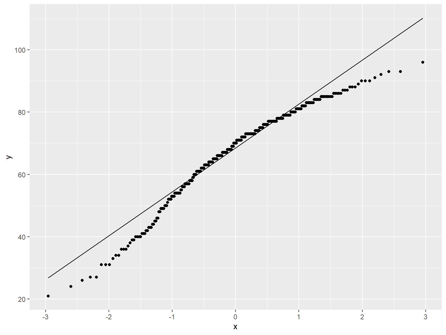
ggplot(exam_data,
       aes(sample = ENGLISH)) +
  stat_qq() +
  stat_qq_line()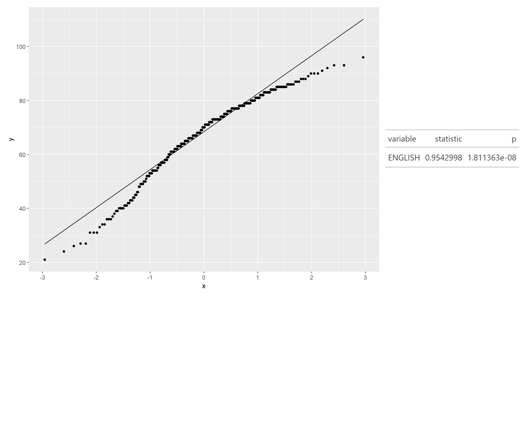

Plot

Code

qq <- ggplot(exam_data,
             aes(sample = ENGLISH)) +
  stat_qq() +
  stat_qq_line()

sw_t <- exam_data %>% shapiro_test(ENGLISH) %>% gt()

tmp <- tempfile(fileext = ".png")
gtsave(sw_t, tmp)
table_png <- png::readPNG(tmp, native = TRUE)

qq + table_png